Presenting: Andrei Kolmogorov
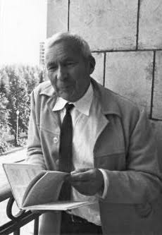
There are mathematicians who solve problems. And there are mathematicians who change the way everyone else asks questions. Andrei Nikolaevich Kolmogorov was the second kind.
He was born in 1903 in Tambov, Russia, and died in 1987 in Moscow, having lived through nearly the entire twentieth century and shaped a significant part of it. His contributions are unusual in their breadth: he provided the axiomatic foundations of modern probability theory in 1933, the framework underlying modern probability theory and much of mathematical statistics. He worked on turbulence, classical mechanics, topology, stochastic processes, and intuitionistic logic. He was not a specialist drilling deeper into one narrow problem. He moved between fields and reorganized the questions inside them.
The work that puts his name in this article came relatively late in his career. In 1965, when he was already one of the most respected mathematicians in the world, he published a short, dense paper: “Three Approaches to the Quantitative Definition of Information.” The central idea sounds almost trivial when stated informally: the complexity of an object can be measured by the length of the shortest program capable of reproducing it. The consequences are not trivial at all.
That became what we now call Kolmogorov complexity, and it changes a surprisingly basic question. Instead of asking how much information does a source produce, we can ask how much irreducible information is contained in this particular object.
The problem before Kolmogorov
To understand what changed, it helps to start with Claude Shannon.
In 1948, Shannon published A Mathematical Theory of Communication and introduced entropy as a measure of the average uncertainty of an information source. Given a random variable X, his measure:
\[H(X) = -\sum_x P(x) \log_2 P(x)\]captures the expected information produced by that source. Shannon was solving an engineering problem: if messages are generated according to some probability distribution, how efficiently can they be encoded and transmitted? It was a theory of distributions, probabilities, and averages.
The problem is what it cannot do. Give me one specific binary sequence:
010101010101010101010101010101...
and another:
110100011101001011000101101101...
Both may be the same length. Knowing that length tells us nothing about whether one contains a simple generative pattern and the other does not. Shannon information can assign a value to a particular outcome when a probability distribution is known, but that still requires a model of the source. Kolmogorov wanted something different. He wanted to say something about an individual object without first assuming the distribution that generated it. And that required changing the question completely.
The shortest possible description
Suppose there exists a universal computer U. For some object x, consider every possible program that makes U output x and halt. Some programs will be unnecessarily long, some will contain redundant instructions. One of them will be shortest. Kolmogorov complexity is the length of that shortest description:
\[K_U(x) = \min_{p:\, U(p)=x} |p|\]where x is the object, p is a program, U is a universal computing machine, and |p| is the length of the program. The important word is not program. It is shortest. We are asking for the most compressed complete explanation of the object that computation allows.
What this looks like in practice. Take a string of ten thousand zeros. Writing the full string requires ten thousand symbols, but a much shorter description exists: “print ‘0’ ten thousand times.” The object is large. Its description is small. The same goes for an alternating sequence, 010101 repeated five thousand times: “repeat ‘01’ five thousand times.” Still very short. Both have very low Kolmogorov complexity.
Now take a sufficiently long string sampled from an ideal random source. Most such strings will have no substantially shorter description than the string itself. There are simply not enough short programs to describe all long strings. For the typical random string, the best description is essentially “print 110100011…” and nothing more. In algorithmic information theory, this is the central connection between incompressibility and randomness: a string is algorithmically random when it has no significantly shorter effective description.
The example I find most useful is π. Its digits look irregular: 3.14159265358979… no repeating block, no apparent pattern. If I showed you a long fragment without context, it could look like noise. But there is a short algorithm behind it. We do not need to store every digit individually, only an algorithm for computing pi and an instruction for how many digits we want. For the first n digits, the description grows far more slowly than the sequence:
\[K(\pi_{1:n}) \leq K(n) + c\]for some fixed constant c representing the algorithm. The appearance of disorder is not the same as irreducible disorder. Something can look random while being generated by a short rule. And something can be genuinely incompressible even after an exhaustive search for patterns inside it.
Randomness is not structure
This is where the theory is easy to misread.
Consider three objects. A string of zeros: very compressible, very low complexity. The first billion digits of pi: still generated by a compact rule, low complexity relative to its enormous size. A billion genuinely random bits: no shorter description exists, very high complexity. Now the uncomfortable question: which of these contains the richest structure? The random string has the highest Kolmogorov complexity, yet it may be the least interesting of the three. Pure noise is difficult to describe precisely because there is no reusable structure inside it.
Kolmogorov complexity measures description length. It does not directly measure organization, sophistication, causal history, or what we casually call depth. Randomness and organized complexity are not the same thing, and treating high K as a sign of rich structure is a mistake.
Description length is not depth. Charles Bennett developed a concept that helps separate these ideas: logical depth. Imagine two objects with similarly short descriptions. One can be generated almost immediately. The other requires an enormous amount of computation before it appears. Their descriptions may be comparable in length. Their computational histories are completely different. Logical depth asks, roughly, how much computational work is required to generate an object from a sufficiently compressed description. This separates two distinct questions: how short is the explanation, and how much computation does that explanation unfold into?
That distinction matters whenever simple rules generate extraordinarily complicated trajectories, which is exactly what happens in biological systems, dynamical systems, and evolution. A cellular automaton may have a tiny rule. Its state after millions of iterations may encode a long computational history. Kolmogorov gives us one dimension of complexity. Not every dimension.
Solomonoff, Kolmogorov, Chaitin
Kolmogorov did not arrive at these ideas alone.
Ray Solomonoff’s work preceded Kolmogorov’s 1965 formulation and approached closely related ideas from the problem of inductive inference. Between 1960 and 1964, he developed what became known as algorithmic probability and Solomonoff induction. His question was: if we do not know the true process generating our observations, is there a universal way to assign probabilities to possible explanations? His answer linked prediction to program length. Short programs receive greater prior weight than long ones. In simplified form, the weighting looks like:
\[P(x) \propto \sum_{p:\, U(p)=x} 2^{-|p|}\]He was building a universal theory of inductive inference. Kolmogorov’s 1965 formulation, arriving from a different direction, became the standard reference point for what is now commonly called Kolmogorov complexity. He was not interested in prediction but in definition. He wanted a rigorous characterization of the information in an individual object and a precise meaning for randomness.
Gregory Chaitin independently developed closely related ideas during the same period, then pushed them toward the foundations of mathematics and computability. He connected program-size complexity with Gödel incompleteness and the halting problem, and introduced his Omega number, the halting probability of a universal prefix-free machine. Its digits are mathematically defined and yet algorithmically irreducible. The broader field that emerged from these ideas is now known as algorithmic information theory, with Solomonoff, Kolmogorov, and Chaitin generally recognized as foundational figures.
The limits of the idea
Why K(x) cannot be computed. Here we have to be direct. Kolmogorov complexity is not computable in general. Not in the sense of being very hard. In the sense that no algorithm exists that accepts every possible string x, returns its exact K(x), and always terminates.
Suppose we find a short program that outputs x. How do we prove that no shorter program does? We would need to inspect all shorter candidate programs, some of which may run for an arbitrarily long time before halting. And there is no general algorithm capable of deciding whether an arbitrary program will eventually halt. We have reached the halting problem. The shortest-description idea gives us an elegant mathematical quantity, and then computability theory immediately prevents us from calculating it exactly. That tension is not a defect in the theory. It is one of its most important results.
Does the programming language matter? There is an obvious question with the definition: if complexity is the size of the shortest program, surely the result depends on the programming language. A Python program may be shorter than the equivalent C program. Does that make complexity arbitrary? Not completely. The invariance theorem provides the essential answer. For two universal description languages U₁ and U₂, their complexity measures differ by at most a fixed additive constant:
\[|K_{U_1}(x) - K_{U_2}(x)| \leq c\]where c depends on the languages, not on x. Why? Because one universal machine can simulate another, and the simulator has some fixed length. Once that cost is paid, descriptions can be translated. For short objects the constant may matter enormously. But asymptotically, for sufficiently large objects, the fundamental notion survives the choice of universal language. That is one reason the theory works at all.
Compression is only a proxy. What you can do is build computable descriptions that act as practical proxies. Any real compression algorithm, gzip, bzip2, LZMA, gives you an upper bound on the Kolmogorov complexity of whatever you feed it. Call the compressed length C(x). If the decompressor plus the compressed file reconstructs x, we have found one valid description:
\[K(x) \leq C(x) + c\]But if gzip compresses a file to 200 kilobytes, that does not mean K(x) equals 200 KB. It means gzip found a description of approximately that size. A different compressor may find something shorter. And we cannot know in general how far our compressor is from the true shortest description. Compressed size is observable. Kolmogorov complexity is the theoretical limit. Practical compression reveals the structure detectable by a particular compressor, nothing more.
When two objects share information
NCD. If two objects share structure, describing them together may require less information than describing them independently. That intuition appears in the Normalized Compression Distance:
\[NCD(x, y) = \frac{C(xy) - \min(C(x), C(y))}{\max(C(x), C(y))}\]where C(x) and C(y) are the compressed sizes of x and y separately, and C(xy) is the compressed size of their concatenation. If x contains patterns useful for describing y, the compressor may reuse some of that structure. The method does not necessarily require handcrafted feature extraction, although the representation given to the compressor still matters enormously. That dependence on representation is not a minor detail, and it connects directly with the invariance theorem: what the theorem guarantees in theory, and what happens with a practical compressor and a specific encoding, are not the same thing. NCD has been explored in text classification, biological sequence comparison, malware detection, clustering, and authorship attribution. What makes it useful is the generality of the question it asks: does knowing one object help compress the other?
Algorithmic mutual information. There is a more fundamental version of the same idea. Algorithmic information theory gives us a notion analogous to mutual information:
\[I(x : y) \approx K(x) + K(y) - K(x, y)\]This formula captures the intuition: how much shorter can two objects be described together than separately? If they have almost nothing in common, K(x, y) ≈ K(x) + K(y) and the shared information approaches zero. If substantial structure is reusable, K(x, y) is smaller than the sum and the shared information grows. The formula above is a useful starting point, but the formal definitions involve subtleties. A more precise treatment uses the conditional form K(x|y*), where y* is the shortest description of y, and the quantities hold up to additive or logarithmic terms depending on the variant used. Two objects do not need to be numerically close to share information in this sense. They need to share description. That becomes interesting whenever the same hidden mechanism generates observations that look very different on the surface.
From description length to learning
MDL. Jorma Rissanen carried related ideas into statistical modeling through the Minimum Description Length principle (Rissanen, 1978). Suppose we have a dataset D and a model M. A model can explain the data, but the model itself also requires information to describe. So instead of minimizing only prediction error, we consider:
\[L(M) + L(D \mid M)\]Here L should be understood as codelength under a specified coding scheme, not merely the physical size or parameter count of the model. A model that memorizes every observation fits perfectly but becomes expensive to describe. A model that is too simple has a short description but leaves much of the data unexplained. MDL searches for the balance: the model that gives the shortest total description of model plus unexplained data. That is a more interesting version of simplicity than just “choose the smallest model.”
Learning as compression. This gives us another way of looking at machine learning. If a dataset contains no regularities, there is little to learn. A model cannot substantially reduce the description of the data. But if the observations contain repeated structure, dependencies, or stable generative mechanisms, a model may capture them, and then:
\[L(M) + L(D \mid M) < L(D)\]Something has been compressed. A model that merely memorizes data stores observations. A model that generalizes has captured something that applies beyond individual examples. But compression of the training set alone is not enough. A representation becomes more interesting when the structure it captures remains useful on data it was not constructed to encode. That distinction, between compressing what you were given and discovering structure that transfers, is one of the central open questions in machine learning.
RL. Reinforcement learning introduces an interesting case. An agent interacts with an environment, observes states, takes actions, receives rewards, and attempts to maximize expected cumulative reward:
\[\max_\pi \mathbb{E}_\pi \left[ \sum_{t=0}^{T} \gamma^t r_t \right]\]The standard formulation says nothing about the descriptive complexity of the policy the agent discovers. Suppose two policies obtain comparable reward. One requires a highly complicated collection of exceptions. Another is governed by a compact rule that works across many states. Should we treat them as equivalent? Not necessarily. As a thought experiment, one could introduce a description-length penalty alongside the reward:
\[J(\pi) = \mathbb{E}[R] - \lambda L(\pi)\]This is not a standard formulation derived directly from Kolmogorov complexity. It is an open line of inquiry. And it immediately creates another problem: simple does not mean aligned. A catastrophically bad policy can be extremely simple, “repeat the exploit forever.” So minimizing policy complexity alone cannot solve reward hacking or specification gaming. The more interesting question is the relationship between K(π), K(E), K(R), and the information shared between a policy, its environment, and the behavior we actually intended. That is not a solved problem. It is a useful one.
What complexity does — and does not — mean
Kolmogorov complexity is powerful partly because the definition is so general. That generality also makes it easy to ask it to do too much.
The concepts that initially looked similar have now separated:
| Object | Description length | Apparent disorder | Computational depth |
|---|---|---|---|
| Repeated zeros | Low | Low | Low |
| Digits of pi | Low relative to length | High | Potentially nontrivial |
| Random bits | High | High | Typically shallow |
| Evolved or adaptive system | Variable | Variable | Potentially high |
A random object can have very high Kolmogorov complexity without being intelligent. A simple rule can generate an enormously complicated pattern without the rule itself being complicated. A short description does not tell us that an object is useful, meaningful, causal, robust, or easy to predict. A long description does not tell us that an object contains rich organization. Noise is the obvious counterexample.
And there is a distinction that deserves to be made explicit: a system can have a compact generative description and still be difficult to predict far into the future. Compressibility and predictability are related questions, not equivalent ones. Knowing the rule does not always mean you can skip the computation.
The correct lesson is not “everything interesting is compression.” It is narrower: description length gives us a rigorous way to distinguish what must be specified from what can be generated from structure. That is already an extraordinary tool.
For centuries, science has depended on a particular instinct. A theory that explains many observations using a small number of principles is preferable to a catalogue containing one independent explanation for every observation. Newton did not need one law for every falling object. Darwin did not need an independent mechanism for every species. Maxwell did not need separate equations for every electromagnetic phenomenon. Science searches for reusable explanation. Kolmogorov complexity gives one rigorous mathematical form to that intuition. Not the only one, and not one that can always be calculated, but one that forces a precise question: how much of this object is genuine irreducible detail, and how much can be generated from a shorter description?
Kolmogorov did not answer all of these. That is not why his work matters. He changed the language in which they can be asked.
Questions worth investigating
Compression and learning
- If a model compresses its training data extremely well, has it discovered transferable structure or merely built a sophisticated form of memorization? What additional conditions would distinguish the two?
- If a representation learned from one dataset significantly reduces the description length of a previously unseen dataset, can that reduction serve as a useful measure of generalization? How would it compare with conventional validation error?
- Kolmogorov complexity is uncomputable. Real compressors detect only particular forms of redundancy. How sensitive are compression-based conclusions to the compressor, encoding, and representation chosen? And when do those differences become scientifically significant?
Shared structure
- Could practical approximations of algorithmic mutual information identify systems produced by related mechanisms even when their raw observations look very different? What representation would make this possible?
- Finite datasets almost always contain accidental regularities. How much apparent compressibility should count as evidence of genuine structure rather than coincidence? How does this interact with sample size?
Complex systems
- A short program can generate an object requiring enormous computational effort. A random string can have maximal description length but almost no meaningful internal organization. Can logical depth or related measures provide a better account of what we intuitively call complex systems?
- Many systems have simple local rules and complicated macroscopic behavior. At what level should complexity be measured: the microscopic state, the generative rule, the emergent patterns, or the history required to produce them?
Reinforcement learning
- If two policies produce similar reward, should preference be given to the one with the shorter effective description? Under what conditions would that improve robustness or transfer, and under what conditions would it simply favor a simple exploit?
- Could overly complicated reward specifications signal that we are encoding examples rather than capturing the intended objective? Conversely, can a reward function be too simple to constrain the behavior we actually care about?
- Instead of asking only how complex a policy is, could we ask how much information about the environment the policy contains, something like I(π:E)? Could this help distinguish adaptive behavior from memorized behavior?
Representation and description
- If Kolmogorov complexity depends on representation only up to an additive constant in theory, why does representation matter so much in practical compression-based methods? Where exactly does the gap between the invariance theorem and empirical sensitivity open up?
- Can a system become more predictable without becoming substantially more compressible, or more compressible without becoming easier to predict? What does the gap between compression and prediction reveal about the structure of the system?
- When we say an object has a short description, that description presupposes a machine and a language. The invariance theorem resolves part of this problem asymptotically, but in practice the representation encodes prior knowledge. How much of the apparent simplicity belongs to the object, and how much belongs to the descriptive language we chose?
In a nutshell
Imagine three long walls made of tiles. One is all white. One alternates black and white. One has no obvious pattern. All three may contain the same number of tiles, but they do not require the same amount of information to describe.
Kolmogorov complexity asks a simple question: what is the shortest complete description that can reproduce this object?
A large object can have a short description. A random-looking object may come from a simple rule. And a truly irregular object may have no shortcut at all.
That is the core idea.
References
Bennett, C. H. (1988). Logical depth and physical complexity. In R. Herken (Ed.), The Universal Turing Machine: A Half-Century Survey. Oxford University Press.
Chaitin, G. J. (1966). On the length of programs for computing finite binary sequences. Journal of the ACM, 13(4), 547–569.
Cilibrasi, R., & Vitányi, P. M. B. (2005). Clustering by compression. IEEE Transactions on Information Theory, 51(4), 1523–1545.
Kolmogorov, A. N. (1965). Three approaches to the quantitative definition of information. Problems of Information Transmission, 1(1), 1–7.
Li, M., & Vitányi, P. M. B. (2008). An Introduction to Kolmogorov Complexity and Its Applications (3rd ed.). Springer.
Rissanen, J. (1978). Modeling by shortest data description. Automatica, 14(5), 465–471.
Shannon, C. E. (1948). A mathematical theory of communication. Bell System Technical Journal, 27, 379–423, 623–656.
Solomonoff, R. J. (1964). A formal theory of inductive inference. Information and Control, 7(1–2), 1–22, 224–254.